# Marigold Computer Vision
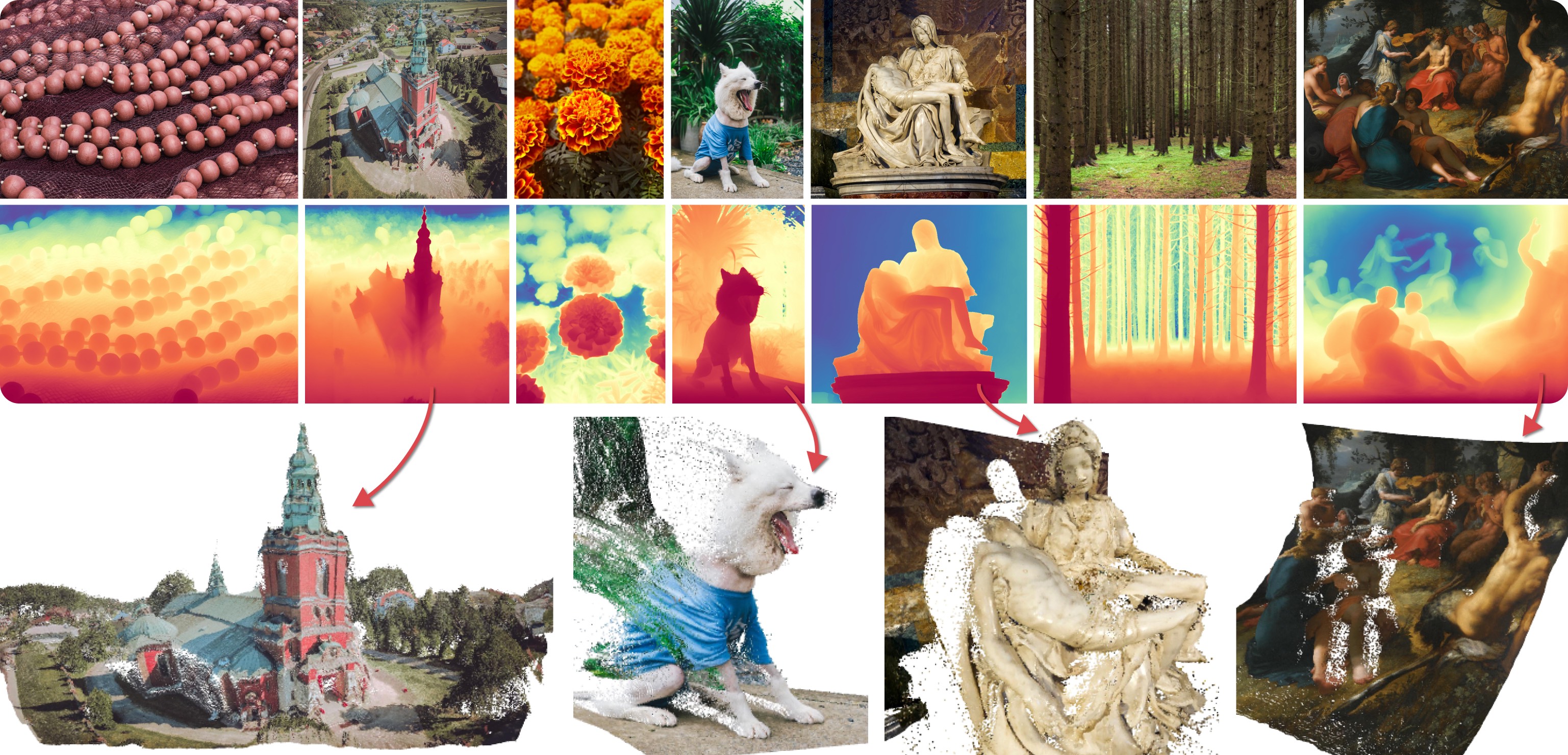
Marigold was proposed in
[Repurposing Diffusion-Based Image Generators for Monocular Depth Estimation](https://huggingface.co/papers/2312.02145),
a CVPR 2024 Oral paper by
[Bingxin Ke](http://www.kebingxin.com/),
[Anton Obukhov](https://www.obukhov.ai/),
[Shengyu Huang](https://shengyuh.github.io/),
[Nando Metzger](https://nandometzger.github.io/),
[Rodrigo Caye Daudt](https://rcdaudt.github.io/), and
[Konrad Schindler](https://scholar.google.com/citations?user=FZuNgqIAAAAJ&hl=en).
The core idea is to **repurpose the generative prior of Text-to-Image Latent Diffusion Models (LDMs) for traditional
computer vision tasks**.
This approach was explored by fine-tuning Stable Diffusion for **Monocular Depth Estimation**, as demonstrated in the
teaser above.
Marigold was later extended in the follow-up paper,
[Marigold: Affordable Adaptation of Diffusion-Based Image Generators for Image Analysis](https://huggingface.co/papers/2312.02145),
authored by
[Bingxin Ke](http://www.kebingxin.com/),
[Kevin Qu](https://www.linkedin.com/in/kevin-qu-b3417621b/?locale=en_US),
[Tianfu Wang](https://tianfwang.github.io/),
[Nando Metzger](https://nandometzger.github.io/),
[Shengyu Huang](https://shengyuh.github.io/),
[Bo Li](https://www.linkedin.com/in/bobboli0202/),
[Anton Obukhov](https://www.obukhov.ai/), and
[Konrad Schindler](https://scholar.google.com/citations?user=FZuNgqIAAAAJ&hl=en).
This work expanded Marigold to support new modalities such as **Surface Normals** and **Intrinsic Image Decomposition**
(IID), introduced a training protocol for **Latent Consistency Models** (LCM), and demonstrated **High-Resolution** (HR)
processing capability.
> [!TIP]
> The early Marigold models (`v1-0` and earlier) were optimized for best results with at least 10 inference steps.
> LCM models were later developed to enable high-quality inference in just 1 to 4 steps.
> Marigold models `v1-1` and later use the DDIM scheduler to achieve optimal
> results in as few as 1 to 4 steps.
## Available Pipelines
Each pipeline is tailored for a specific computer vision task, processing an input RGB image and generating a
corresponding prediction.
Currently, the following computer vision tasks are implemented:
| Pipeline | Recommended Model Checkpoints | Spaces (Interactive Apps) | Predicted Modalities |
|---------------------------------------------------------------------------------------------------------------------------------------------------|---------------------------------------------------------------------------------------------------------------------------------------------------------------------------------------------------------|:------------------------------------------------------------------------------------:|------------------------------------------------------------------------------------------------------------------------------------------------------------------------------------|
| [MarigoldDepthPipeline](https://github.com/huggingface/diffusers/blob/main/src/diffusers/pipelines/marigold/pipeline_marigold_depth.py) | [prs-eth/marigold-depth-v1-1](https://huggingface.co/prs-eth/marigold-depth-v1-1) | [Depth Estimation](https://huggingface.co/spaces/prs-eth/marigold) | [Depth](https://en.wikipedia.org/wiki/Depth_map), [Disparity](https://en.wikipedia.org/wiki/Binocular_disparity) |
| [MarigoldNormalsPipeline](https://github.com/huggingface/diffusers/blob/main/src/diffusers/pipelines/marigold/pipeline_marigold_normals.py) | [prs-eth/marigold-normals-v1-1](https://huggingface.co/prs-eth/marigold-normals-v1-1) | [Surface Normals Estimation](https://huggingface.co/spaces/prs-eth/marigold-normals) | [Surface normals](https://en.wikipedia.org/wiki/Normal_mapping) |
| [MarigoldIntrinsicsPipeline](https://github.com/huggingface/diffusers/blob/main/src/diffusers/pipelines/marigold/pipeline_marigold_intrinsics.py) | [prs-eth/marigold-iid-appearance-v1-1](https://huggingface.co/prs-eth/marigold-iid-appearance-v1-1),
[prs-eth/marigold-iid-lighting-v1-1](https://huggingface.co/prs-eth/marigold-iid-lighting-v1-1) | [Intrinsic Image Decomposition](https://huggingface.co/spaces/prs-eth/marigold-iid) | [Albedo](https://en.wikipedia.org/wiki/Albedo), [Materials](https://www.n.aiq3d.com/wiki/roughnessmetalnessao-map), [Lighting](https://en.wikipedia.org/wiki/Diffuse_reflection) |
## Available Checkpoints
All original checkpoints are available under the [PRS-ETH](https://huggingface.co/prs-eth/) organization on Hugging Face.
They are designed for use with diffusers pipelines and the [original codebase](https://github.com/prs-eth/marigold), which can also be used to train
new model checkpoints.
The following is a summary of the recommended checkpoints, all of which produce reliable results with 1 to 4 steps.
| Checkpoint | Modality | Comment |
|-----------------------------------------------------------------------------------------------------|--------------|--------------------------------------------------------------------------------------------------------------------------------------------------------------------------------------|
| [prs-eth/marigold-depth-v1-1](https://huggingface.co/prs-eth/marigold-depth-v1-1) | Depth | Affine-invariant depth prediction assigns each pixel a value between 0 (near plane) and 1 (far plane), with both planes determined by the model during inference. |
| [prs-eth/marigold-normals-v0-1](https://huggingface.co/prs-eth/marigold-normals-v0-1) | Normals | The surface normals predictions are unit-length 3D vectors in the screen space camera, with values in the range from -1 to 1. |
| [prs-eth/marigold-iid-appearance-v1-1](https://huggingface.co/prs-eth/marigold-iid-appearance-v1-1) | Intrinsics | InteriorVerse decomposition is comprised of Albedo and two BRDF material properties: Roughness and Metallicity. |
| [prs-eth/marigold-iid-lighting-v1-1](https://huggingface.co/prs-eth/marigold-iid-lighting-v1-1) | Intrinsics | HyperSim decomposition of an image $I$ is comprised of Albedo $A$, Diffuse shading $S$, and Non-diffuse residual $R$: $I = A*S+R$. |
> [!TIP]
> Make sure to check out the Schedulers [guide](../../using-diffusers/schedulers) to learn how to explore the tradeoff
> between scheduler speed and quality, and see the [reuse components across pipelines](../../using-diffusers/loading#reuse-a-pipeline) section to learn how to
> efficiently load the same components into multiple pipelines.
> Also, to know more about reducing the memory usage of this pipeline, refer to the ["Reduce memory usage"] section
> [here](./stable_diffusion/svd#reduce-memory-usage).
> [!WARNING]
> Marigold pipelines were designed and tested with the scheduler embedded in the model checkpoint.
> The optimal number of inference steps varies by scheduler, with no universal value that works best across all cases.
> To accommodate this, the `num_inference_steps` parameter in the pipeline's `__call__` method defaults to `None` (see the
> API reference).
> Unless set explicitly, it inherits the value from the `default_denoising_steps` field in the checkpoint configuration
> file (`model_index.json`).
> This ensures high-quality predictions when invoking the pipeline with only the `image` argument.
The examples below are mostly given for depth prediction, but they can be universally applied to other supported
modalities.
We showcase the predictions using the same input image of Albert Einstein generated by Midjourney.
This makes it easier to compare visualizations of the predictions across various modalities and checkpoints.
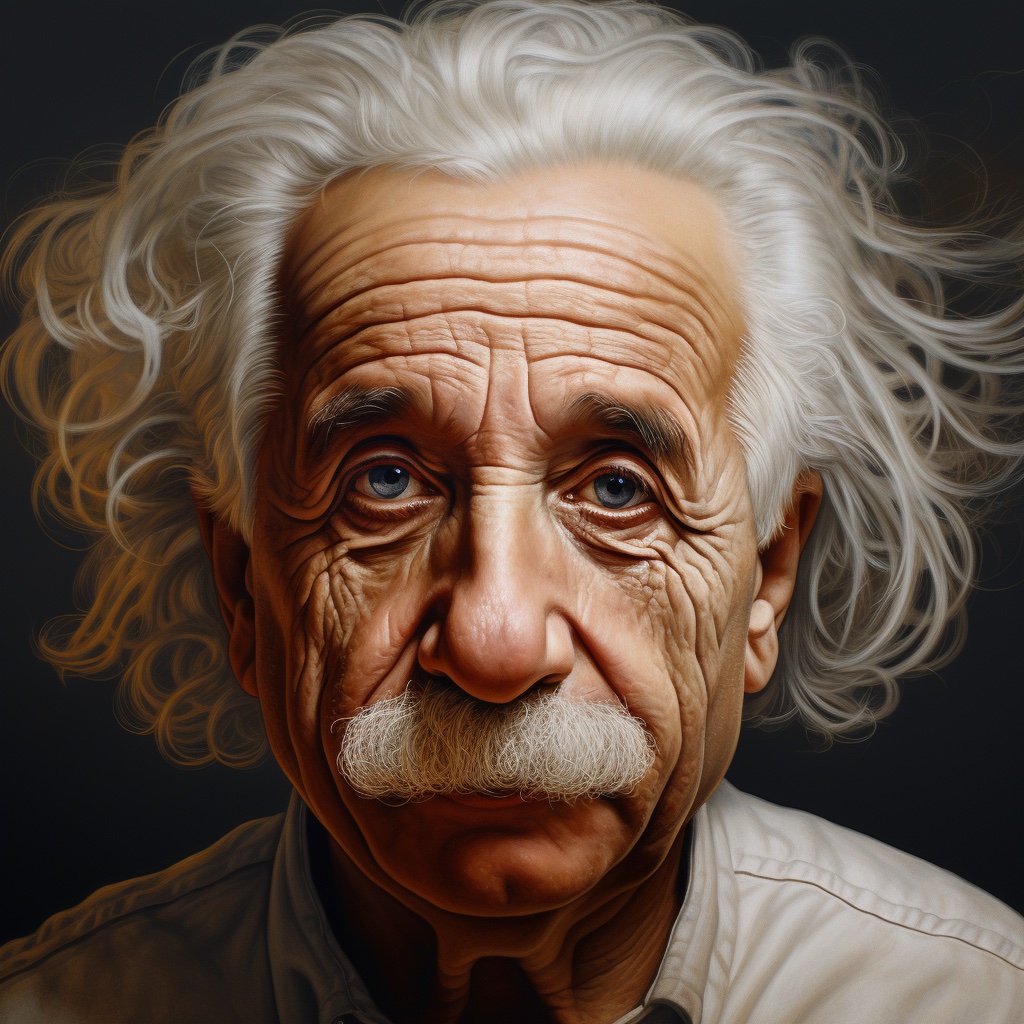 Example input image for all Marigold pipelines
## Depth Prediction
To get a depth prediction, load the `prs-eth/marigold-depth-v1-1` checkpoint into [`MarigoldDepthPipeline`],
put the image through the pipeline, and save the predictions:
```python
import diffusers
import torch
pipe = diffusers.MarigoldDepthPipeline.from_pretrained(
"prs-eth/marigold-depth-v1-1", variant="fp16", dtype=torch.float16
).to("cuda")
image = diffusers.utils.load_image("https://marigoldmonodepth.github.io/images/einstein.jpg")
depth = pipe(image)
vis = pipe.image_processor.visualize_depth(depth.prediction)
vis[0].save("einstein_depth.png")
depth_16bit = pipe.image_processor.export_depth_to_16bit_png(depth.prediction)
depth_16bit[0].save("einstein_depth_16bit.png")
```
The [`~pipelines.marigold.marigold_image_processing.MarigoldImageProcessor.visualize_depth`] function applies one of
[matplotlib's colormaps](https://matplotlib.org/stable/users/explain/colors/colormaps.html) (`Spectral` by default) to map the predicted pixel values from a single-channel `[0, 1]`
depth range into an RGB image.
With the `Spectral` colormap, pixels with near depth are painted red, and far pixels are blue.
The 16-bit PNG file stores the single channel values mapped linearly from the `[0, 1]` range into `[0, 65535]`.
Below are the raw and the visualized predictions. The darker and closer areas (mustache) are easier to distinguish in
the visualization.
 Predicted depth (16-bit PNG)
 Predicted depth visualization (Spectral)
## Surface Normals Estimation
Load the `prs-eth/marigold-normals-v1-1` checkpoint into [`MarigoldNormalsPipeline`], put the image through the
pipeline, and save the predictions:
```python
import diffusers
import torch
pipe = diffusers.MarigoldNormalsPipeline.from_pretrained(
"prs-eth/marigold-normals-v1-1", variant="fp16", dtype=torch.float16
).to("cuda")
image = diffusers.utils.load_image("https://marigoldmonodepth.github.io/images/einstein.jpg")
normals = pipe(image)
vis = pipe.image_processor.visualize_normals(normals.prediction)
vis[0].save("einstein_normals.png")
```
The [`~pipelines.marigold.marigold_image_processing.MarigoldImageProcessor.visualize_normals`] maps the three-dimensional
prediction with pixel values in the range `[-1, 1]` into an RGB image.
The visualization function supports flipping surface normals axes to make the visualization compatible with other
choices of the frame of reference.
Conceptually, each pixel is painted according to the surface normal vector in the frame of reference, where `X` axis
points right, `Y` axis points up, and `Z` axis points at the viewer.
Below is the visualized prediction:
 Predicted surface normals visualization
In this example, the nose tip almost certainly has a point on the surface, in which the surface normal vector points
straight at the viewer, meaning that its coordinates are `[0, 0, 1]`.
This vector maps to the RGB `[128, 128, 255]`, which corresponds to the violet-blue color.
Similarly, a surface normal on the cheek in the right part of the image has a large `X` component, which increases the
red hue.
Points on the shoulders pointing up with a large `Y` promote green color.
## Intrinsic Image Decomposition
Marigold provides two models for Intrinsic Image Decomposition (IID): "Appearance" and "Lighting".
Each model produces Albedo maps, derived from InteriorVerse and Hypersim annotations, respectively.
- The "Appearance" model also estimates Material properties: Roughness and Metallicity.
- The "Lighting" model generates Diffuse Shading and Non-diffuse Residual.
Here is the sample code saving predictions made by the "Appearance" model:
```python
import diffusers
import torch
pipe = diffusers.MarigoldIntrinsicsPipeline.from_pretrained(
"prs-eth/marigold-iid-appearance-v1-1", variant="fp16", dtype=torch.float16
).to("cuda")
image = diffusers.utils.load_image("https://marigoldmonodepth.github.io/images/einstein.jpg")
intrinsics = pipe(image)
vis = pipe.image_processor.visualize_intrinsics(intrinsics.prediction, pipe.target_properties)
vis[0]["albedo"].save("einstein_albedo.png")
vis[0]["roughness"].save("einstein_roughness.png")
vis[0]["metallicity"].save("einstein_metallicity.png")
```
Another example demonstrating the predictions made by the "Lighting" model:
```python
import diffusers
import torch
pipe = diffusers.MarigoldIntrinsicsPipeline.from_pretrained(
"prs-eth/marigold-iid-lighting-v1-1", variant="fp16", dtype=torch.float16
).to("cuda")
image = diffusers.utils.load_image("https://marigoldmonodepth.github.io/images/einstein.jpg")
intrinsics = pipe(image)
vis = pipe.image_processor.visualize_intrinsics(intrinsics.prediction, pipe.target_properties)
vis[0]["albedo"].save("einstein_albedo.png")
vis[0]["shading"].save("einstein_shading.png")
vis[0]["residual"].save("einstein_residual.png")
```
Both models share the same pipeline while supporting different decomposition types.
The exact decomposition parameterization (e.g., sRGB vs. linear space) is stored in the
`pipe.target_properties` dictionary, which is passed into the
[`~pipelines.marigold.marigold_image_processing.MarigoldImageProcessor.visualize_intrinsics`] function.
Below are some examples showcasing the predicted decomposition outputs.
All modalities can be inspected in the
[Intrinsic Image Decomposition](https://huggingface.co/spaces/prs-eth/marigold-iid) Space.
 Predicted albedo ("Appearance" model)
 Predicted diffuse shading ("Lighting" model)
## Speeding up inference
The above quick start snippets are already optimized for quality and speed, loading the checkpoint, utilizing the
`fp16` variant of weights and computation, and performing the default number (4) of denoising diffusion steps.
The first step to accelerate inference, at the expense of prediction quality, is to reduce the denoising diffusion
steps to the minimum:
```diff
import diffusers
import torch
pipe = diffusers.MarigoldDepthPipeline.from_pretrained(
"prs-eth/marigold-depth-v1-1", variant="fp16", dtype=torch.float16
).to("cuda")
image = diffusers.utils.load_image("https://marigoldmonodepth.github.io/images/einstein.jpg")
- depth = pipe(image)
+ depth = pipe(image, num_inference_steps=1)
```
With this change, the `pipe` call completes in 280ms on RTX 3090 GPU.
Internally, the input image is first encoded using the Stable Diffusion VAE encoder, followed by a single denoising
step performed by the U-Net.
Finally, the prediction latent is decoded with the VAE decoder into pixel space.
In this setup, two out of three module calls are dedicated to converting between the pixel and latent spaces of the LDM.
Since Marigold's latent space is compatible with Stable Diffusion 2.0, inference can be accelerated by more than 3x,
reducing the call time to 85ms on an RTX 3090, by using a [lightweight replacement of the SD VAE](../models/autoencoder_tiny).
Note that using a lightweight VAE may slightly reduce the visual quality of the predictions.
```diff
import diffusers
import torch
pipe = diffusers.MarigoldDepthPipeline.from_pretrained(
"prs-eth/marigold-depth-v1-1", variant="fp16", dtype=torch.float16
).to("cuda")
+ pipe.vae = diffusers.AutoencoderTiny.from_pretrained(
+ "madebyollin/taesd", dtype=torch.float16
+ ).cuda()
image = diffusers.utils.load_image("https://marigoldmonodepth.github.io/images/einstein.jpg")
depth = pipe(image, num_inference_steps=1)
```
So far, we have optimized the number of diffusion steps and model components. Self-attention operations account for a
significant portion of computations.
Speeding them up can be achieved by using a more efficient attention processor:
```diff
import diffusers
import torch
+ from diffusers.models.attention_processor import AttnProcessor2_0
pipe = diffusers.MarigoldDepthPipeline.from_pretrained(
"prs-eth/marigold-depth-v1-1", variant="fp16", dtype=torch.float16
).to("cuda")
+ pipe.vae.set_attn_processor(AttnProcessor2_0())
+ pipe.unet.set_attn_processor(AttnProcessor2_0())
image = diffusers.utils.load_image("https://marigoldmonodepth.github.io/images/einstein.jpg")
depth = pipe(image, num_inference_steps=1)
```
Finally, as suggested in [Optimizations](../../optimization/fp16#torchcompile), enabling `torch.compile` can further enhance performance depending on
the target hardware.
However, compilation incurs a significant overhead during the first pipeline invocation, making it beneficial only when
the same pipeline instance is called repeatedly, such as within a loop.
```diff
import diffusers
import torch
from diffusers.models.attention_processor import AttnProcessor2_0
pipe = diffusers.MarigoldDepthPipeline.from_pretrained(
"prs-eth/marigold-depth-v1-1", variant="fp16", dtype=torch.float16
).to("cuda")
pipe.vae.set_attn_processor(AttnProcessor2_0())
pipe.unet.set_attn_processor(AttnProcessor2_0())
+ pipe.vae = torch.compile(pipe.vae, mode="reduce-overhead", fullgraph=True)
+ pipe.unet = torch.compile(pipe.unet, mode="reduce-overhead", fullgraph=True)
image = diffusers.utils.load_image("https://marigoldmonodepth.github.io/images/einstein.jpg")
depth = pipe(image, num_inference_steps=1)
```
## Maximizing Precision and Ensembling
Marigold pipelines have a built-in ensembling mechanism combining multiple predictions from different random latents.
This is a brute-force way of improving the precision of predictions, capitalizing on the generative nature of diffusion.
The ensembling path is activated automatically when the `ensemble_size` argument is set greater or equal than `3`.
When aiming for maximum precision, it makes sense to adjust `num_inference_steps` simultaneously with `ensemble_size`.
The recommended values vary across checkpoints but primarily depend on the scheduler type.
The effect of ensembling is particularly well-seen with surface normals:
```diff
import diffusers
pipe = diffusers.MarigoldNormalsPipeline.from_pretrained("prs-eth/marigold-normals-v1-1").to("cuda")
image = diffusers.utils.load_image("https://marigoldmonodepth.github.io/images/einstein.jpg")
- depth = pipe(image)
+ depth = pipe(image, num_inference_steps=10, ensemble_size=5)
vis = pipe.image_processor.visualize_normals(depth.prediction)
vis[0].save("einstein_normals.png")
```
Surface normals, no ensembling
 Surface normals, with ensembling
As can be seen, all areas with fine-grained structurers, such as hair, got more conservative and on average more
correct predictions.
Such a result is more suitable for precision-sensitive downstream tasks, such as 3D reconstruction.
## Frame-by-frame Video Processing with Temporal Consistency
Due to Marigold's generative nature, each prediction is unique and defined by the random noise sampled for the latent
initialization.
This becomes an obvious drawback compared to traditional end-to-end dense regression networks, as exemplified in the
following videos:
 Input video
 Marigold Depth applied to input video frames independently
To address this issue, it is possible to pass `latents` argument to the pipelines, which defines the starting point of
diffusion.
Empirically, we found that a convex combination of the very same starting point noise latent and the latent
corresponding to the previous frame prediction give sufficiently smooth results, as implemented in the snippet below:
```python
import imageio
import diffusers
import torch
from diffusers.models.attention_processor import AttnProcessor2_0
from PIL import Image
from tqdm import tqdm
device = "cuda"
path_in = "https://huggingface.co/spaces/prs-eth/marigold-lcm/resolve/c7adb5427947d2680944f898cd91d386bf0d4924/files/video/obama.mp4"
path_out = "obama_depth.gif"
pipe = diffusers.MarigoldDepthPipeline.from_pretrained(
"prs-eth/marigold-depth-v1-1", variant="fp16", dtype=torch.float16
).to(device)
pipe.vae = diffusers.AutoencoderTiny.from_pretrained(
"madebyollin/taesd", dtype=torch.float16
).to(device)
pipe.unet.set_attn_processor(AttnProcessor2_0())
pipe.vae = torch.compile(pipe.vae, mode="reduce-overhead", fullgraph=True)
pipe.unet = torch.compile(pipe.unet, mode="reduce-overhead", fullgraph=True)
pipe.set_progress_bar_config(disable=True)
with imageio.get_reader(path_in) as reader:
size = reader.get_meta_data()['size']
last_frame_latent = None
latent_common = torch.randn(
(1, 4, 768 * size[1] // (8 * max(size)), 768 * size[0] // (8 * max(size)))
).to(device=device, dtype=torch.float16)
out = []
for frame_id, frame in tqdm(enumerate(reader), desc="Processing Video"):
frame = Image.fromarray(frame)
latents = latent_common
if last_frame_latent is not None:
latents = 0.9 * latents + 0.1 * last_frame_latent
depth = pipe(
frame,
num_inference_steps=1,
match_input_resolution=False,
latents=latents,
output_latent=True,
)
last_frame_latent = depth.latent
out.append(pipe.image_processor.visualize_depth(depth.prediction)[0])
diffusers.utils.export_to_gif(out, path_out, fps=reader.get_meta_data()['fps'])
```
Here, the diffusion process starts from the given computed latent.
The pipeline sets `output_latent=True` to access `out.latent` and computes its contribution to the next frame's latent
initialization.
The result is much more stable now:
Marigold Depth applied to input video frames independently
 Marigold Depth with forced latents initialization
## Marigold for ControlNet
A very common application for depth prediction with diffusion models comes in conjunction with ControlNet.
Depth crispness plays a crucial role in obtaining high-quality results from ControlNet.
As seen in comparisons with other methods above, Marigold excels at that task.
The snippet below demonstrates how to load an image, compute depth, and pass it into ControlNet in a compatible format:
```python
import torch
import diffusers
device = "cuda"
generator = torch.Generator(device=device).manual_seed(2024)
image = diffusers.utils.load_image(
"https://huggingface.co/datasets/huggingface/documentation-images/resolve/main/diffusers/controlnet_depth_source.png"
)
pipe = diffusers.MarigoldDepthPipeline.from_pretrained(
"prs-eth/marigold-depth-v1-1", dtype=torch.float16, variant="fp16"
).to(device)
depth_image = pipe(image, generator=generator).prediction
depth_image = pipe.image_processor.visualize_depth(depth_image, color_map="binary")
depth_image[0].save("motorcycle_controlnet_depth.png")
controlnet = diffusers.ControlNetModel.from_pretrained(
"diffusers/controlnet-depth-sdxl-1.0", dtype=torch.float16, variant="fp16"
).to(device)
pipe = diffusers.StableDiffusionXLControlNetPipeline.from_pretrained(
"SG161222/RealVisXL_V4.0", dtype=torch.float16, variant="fp16", controlnet=controlnet
).to(device)
pipe.scheduler = diffusers.DPMSolverMultistepScheduler.from_config(pipe.scheduler.config, use_karras_sigmas=True)
controlnet_out = pipe(
prompt="high quality photo of a sports bike, city",
negative_prompt="",
guidance_scale=6.5,
num_inference_steps=25,
image=depth_image,
controlnet_conditioning_scale=0.7,
control_guidance_end=0.7,
generator=generator,
).images
controlnet_out[0].save("motorcycle_controlnet_out.png")
```
 Input image
 Depth in the format compatible with ControlNet
 ControlNet generation, conditioned on depth and prompt: "high quality photo of a sports bike, city"
## Quantitative Evaluation
To evaluate Marigold quantitatively in standard leaderboards and benchmarks (such as NYU, KITTI, and other datasets),
follow the evaluation protocol outlined in the paper: load the full precision fp32 model and use appropriate values
for `num_inference_steps` and `ensemble_size`.
Optionally seed randomness to ensure reproducibility.
Maximizing `batch_size` will deliver maximum device utilization.
```python
import diffusers
import torch
device = "cuda"
seed = 2024
generator = torch.Generator(device=device).manual_seed(seed)
pipe = diffusers.MarigoldDepthPipeline.from_pretrained("prs-eth/marigold-depth-v1-1").to(device)
image = diffusers.utils.load_image("https://marigoldmonodepth.github.io/images/einstein.jpg")
depth = pipe(
image,
num_inference_steps=4, # set according to the evaluation protocol from the paper
ensemble_size=10, # set according to the evaluation protocol from the paper
generator=generator,
)
# evaluate metrics
```
## Using Predictive Uncertainty
The ensembling mechanism built into Marigold pipelines combines multiple predictions obtained from different random
latents.
As a side effect, it can be used to quantify epistemic (model) uncertainty; simply specify `ensemble_size` greater
or equal than 3 and set `output_uncertainty=True`.
The resulting uncertainty will be available in the `uncertainty` field of the output.
It can be visualized as follows:
```python
import diffusers
import torch
pipe = diffusers.MarigoldDepthPipeline.from_pretrained(
"prs-eth/marigold-depth-v1-1", variant="fp16", dtype=torch.float16
).to("cuda")
image = diffusers.utils.load_image("https://marigoldmonodepth.github.io/images/einstein.jpg")
depth = pipe(
image,
ensemble_size=10, # any number >= 3
output_uncertainty=True,
)
uncertainty = pipe.image_processor.visualize_uncertainty(depth.uncertainty)
uncertainty[0].save("einstein_depth_uncertainty.png")
```
 Depth uncertainty
 Surface normals uncertainty
 Albedo uncertainty
The interpretation of uncertainty is easy: higher values (white) correspond to pixels, where the model struggles to
make consistent predictions.
- The depth model exhibits the most uncertainty around discontinuities, where object depth changes abruptly.
- The surface normals model is least confident in fine-grained structures like hair and in dark regions such as the
collar area.
- Albedo uncertainty is represented as an RGB image, as it captures uncertainty independently for each color channel,
unlike depth and surface normals. It is also higher in shaded regions and at discontinuities.
## Marigold Depth Prediction API
[[autodoc]] MarigoldDepthPipeline
- __call__
[[autodoc]] pipelines.marigold.pipeline_marigold_depth.MarigoldDepthOutput
[[autodoc]] pipelines.marigold.marigold_image_processing.MarigoldImageProcessor.visualize_depth
## Marigold Normals Estimation API
[[autodoc]] MarigoldNormalsPipeline
- __call__
[[autodoc]] pipelines.marigold.pipeline_marigold_normals.MarigoldNormalsOutput
[[autodoc]] pipelines.marigold.marigold_image_processing.MarigoldImageProcessor.visualize_normals
## Marigold Intrinsic Image Decomposition API
[[autodoc]] MarigoldIntrinsicsPipeline
- __call__
[[autodoc]] pipelines.marigold.pipeline_marigold_intrinsics.MarigoldIntrinsicsOutput
[[autodoc]] pipelines.marigold.marigold_image_processing.MarigoldImageProcessor.visualize_intrinsics