Chunked Diffusion

Introduction

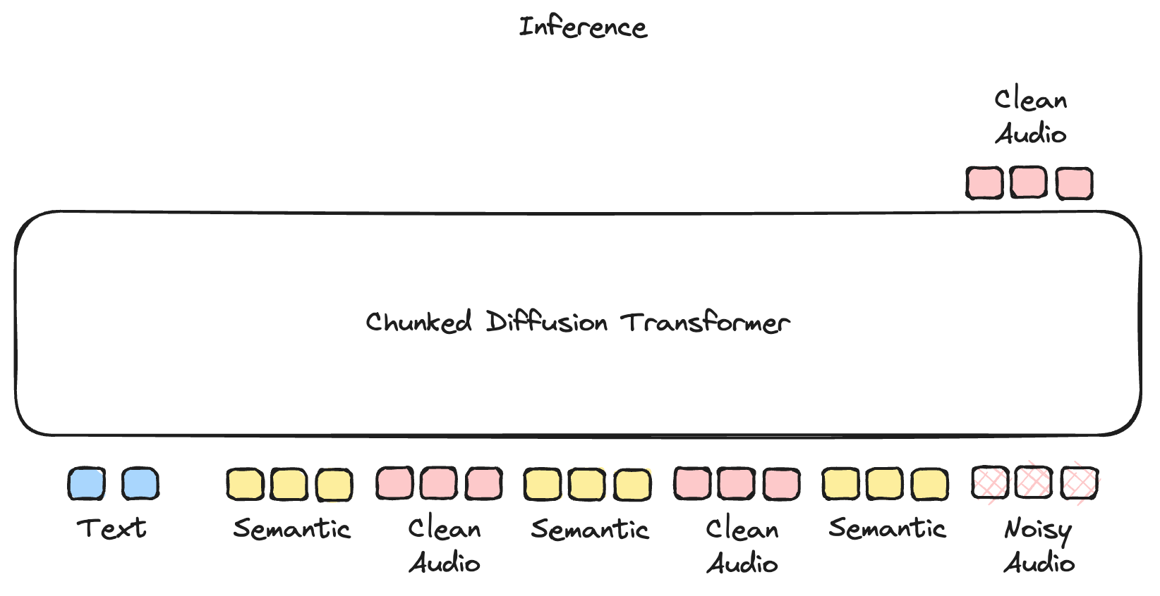
Chunked diffusion is a hybrid of GPT and diffusion architectures, attempting to achieve the best of both worlds. Diffusion models have higher fidelity, but also higher latency. To improve latency, we partition the input sequence into chunks a few seconds long. Tokens can attend to other tokens in the same or preceding chunks. Each chunk is diffused independently and appended to the final result in order. This allows us to stream audio as soon as the first chunk is finished.

Latency

The time to generate a full song with chunked diffusion can be much lower than GPT. GPT generates a single token at a time, and so must make N forward passes to generate N tokens. Chunked diffusion generates C tokens in parallel with S sampling steps, requiring \(\frac{NS}{C}\) forward passes. These forward passes take similar times since both are bottlenecked by moving model weights to SRAM. GPT is run with a large batch size for throughput, which further slows it. Thus chunked diffusion is \(\frac{C}{S}\) times faster than GPT. With a chunk size of 125 and 25 sampling steps this would be 5 times faster. Assuming same sized models. Diffusion models tend to be smaller, increasing the relative speedup.

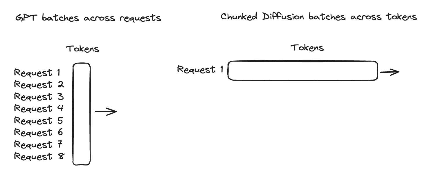
Another way to view this is that in GPT, the compute is spread over many requests in a batch, while in chunked diffusion, it's concentrated on a single request. We'd rather complete a single request quickly than many requests slowly.

Training

It's reasonable to ask why this architecture isn't already popular given the claimed advantages. I believe it's due to the difficulty of training such an architecture efficiently.

Signal Density

To compare different model architectures, let's introduce the concept of "signal density." Signal density represents the ratio of useful training signal to the total amount of data processed. We can express this as:

\[ \text{Signal Density} = \frac{\text{tokens contributing to the} \text{ loss}}{\text{total tokens processed by the model}} \]

In autoregressive models like GPT, each token predicts the next, meaning every token contributes to the loss. This results in a signal density of 1. Similarly, for standard diffusion models, each token predicts its de-noised version, yielding a signal density of 1.

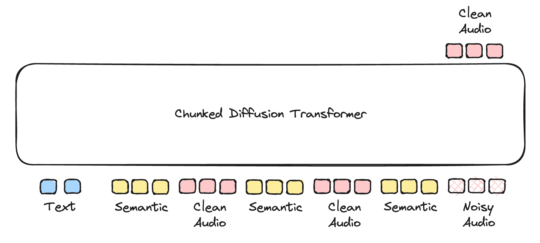⊕ Naive Chunked Diffusion Training Process. Only a single chunk provides training signal.

Calculating the signal density of chunked diffusion is trickier since a noisy chunk must be preceded by clean chunks. A naive approach is to randomly sample a chunk to noise and only compute loss on that single chunk. This gives a signal density of \(\frac{C}{2N}\) For simplicity, we're assuming here that our sequence consists only of audio tokens. In practice, there are also text and semantic tokens, which would further lower the signal per token ratio. since we still pass in all the preceding clean chunks. Since C is much shorter than the total duration N, this is an extremely low signal density.

Smarter Teacher Forcing

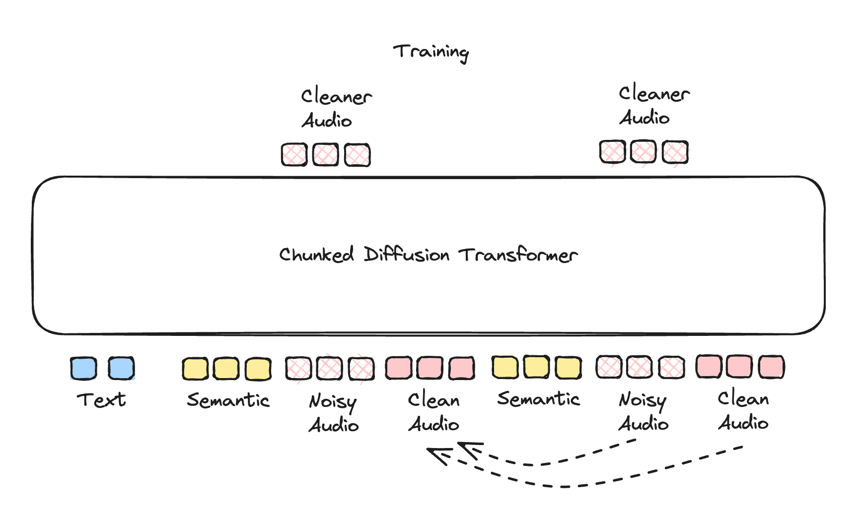⊕ Smarter Chunked Diffusion Training Process. All noisy chunks provide training signal. Chunks attend to previous clean chunks.

We can do better if we interleave clean and noised chunks with a clever attention mask. This mask will allow chunks to only attend to previous clean chunks. Noisy chunks are never attended to by other chunks. In this way we can train on all noisy chunks at once. Our signal density is \(\frac{N}{2N} = \frac{1}{2}\) since we get signal for every noised chunk, but we doubled the sequence by adding the clean chunks. This is a huge improvement which makes training feasible. While 1/2 is a significant improvement, it's still less than the signal density of 1 for standard autoregressive and diffusion models. We discuss this more later.

It's not easy to implement such a custom attention mask. At least, it wasn't until last month. The release of FlexAttention has made it easy to create custom performant attention masks. This is a clear example of tools enabling research.

Note that no attention mask is required at inference time. The query is the last chunk, and the kv's will include the entire past context. This is simply full attention, so we can use flash_attn_with_kvcache with causal=False. This allows us to use flash attention 3 with all its bells and whistles.

Next Steps

Semantic Tokens

Currently the model doesn't predict semantic tokens. This is a big open question. Should semantic be computed with diffusion? Discrete autoregression? Or distilled? If we distill, we can add the loss on the clean chunks to add "free" signal.

Variable Chunk Size

It's not necessary to fix the chunk size. We can train with variable chunk sizes even within a sample. This would allow for precise duration control during infilling.

Improving Signal Density

A signal density of \(\frac{1}{2}\) isn't the best. We can further amortize the cost of predicting clean chunks by predicting more noised chunks with different noise levels. However this blows up our memory requirements.

Diffusion Forcing

Alternatively if we drop the requirement that preceding chunks must be clean, we don't need to compute clean chunks at all (diffusion forcing). This leads to even more natural infilling capabilities.

Longer Contexts

So far we've only trained on 30 second clips. We must scale to full songs, perhaps implementing some form of local attention.